Ballistics Overview · Volume 11
Solving It in Practice & Cheatsheet
Everything in this series converges here: how you turn the physics into a hit. The good news is that a modern solver integrates almost all of it for you — drag, gravity, air density, spin drift, Coriolis, angle. The work that remains is feeding it honest inputs and truing it against reality. This volume is the practical pipeline and a laminate-ready synthesis.
11.1 DOPE — the Ground Truth
DOPE (“data on previous engagements”) is the confirmed record of the actual scope corrections that put rounds on target at known distances, in known conditions. It is the ground truth every solver is ultimately checked against. A solver predicts; DOPE confirms or corrects. The entire truing process below is the disciplined reconciliation of predicted dope against confirmed dope.
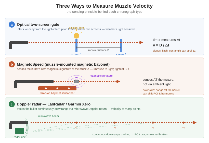
11.2 Chronographs — Three Ways to Measure Velocity
Muzzle velocity is the single most important input to a supersonic firing solution, and there are three ways to measure it.12
- Optical (two-screen gate): infers velocity from the time between two light-interruption events a known distance apart. Weakness: it is sensitive to lighting — clouds, muzzle flash, sun angle, shadows from nearby shooters — so run-to-run consistency can suffer even when the load is genuinely consistent.
- MagnetoSpeed (muzzle-mounted magnetic): a strap-on bayonet-style sensor at the muzzle detects the bullet’s own magnetic signature crossing a fixed zone. Because it senses at the muzzle rather than relying on ambient light, it is largely immune to wind, rain, sun, and nearby blast, and is cited as producing the tightest standard deviations in head-to-head tests. Downside: it hangs off the barrel and can shift point of impact and harmonics while attached.
- Doppler radar (LabRadar, Garmin Xero C1 / C1 Pro): continuously tracks the bullet’s actual flight via microwave Doppler return, so unlike a two-point gate it can report velocity at multiple downrange points — directly useful for BC and drag-curve verification, not just muzzle velocity. LabRadar transmits at lower power (~4.84 dBm, US version) than the newer Garmin Xero C1 Pro (~18.68 dBm), which helps the Xero’s small footprint and lock-on. The Xero is pocket-sized (2.38×3×1.35 in, ~3.5 oz), rated 100–5,000 fps, IPX7, ~2,000 shots per charge. In one 10-shot head-to-head: LabRadar 2767 fps / ES 66 / SD 21.5 versus Garmin Xero 2767.8 fps / ES 71 / SD 21.3 — essentially matching average velocity with broadly similar spread.2 Note per the source: the Xero does not report multi-point downrange velocity the way LabRadar does, which makes downrange BC truing “somewhat harder” with the Xero, “but no more difficult than any traditional velocity measurement method.” These product specs are medium-high confidence (detailed hands-on review); the single head-to-head string is one data point, not a controlled study.
11.3 Truing the Solver
A ballistic solver’s supersonic-range predictions are governed almost entirely by (muzzle velocity × drag curve/BC). You can “true” — back-solve — either variable against confirmed dope, and the trick is to true each one against the range regime where it is the dominant error source.34
Velocity truing. If the trajectory error appears within the fully-supersonic portion of the flight and the drag model is trusted, adjust the solver’s assumed muzzle velocity up or down until predicted drop matches confirmed dope. Applied Ballistics’ Kestrel guidance recommends truing velocity at a range close to — but not past — the transonic transition (a cited guideline is “within 15% of transonic without going over”), because velocity truing loses validity once transonic/subsonic drag uncertainty starts dominating the error.3
BC / drag-scale-factor truing. If the error only shows up in the transonic/subsonic range — the supersonic solution already matches with a good chronographed MV — the fix is to true the drag model instead. The recommended sequence in Applied Ballistics’ materials is roughly: confirm/true velocity first using data around ~600 yd (fully supersonic for most cartridges), then true BC by comparing predicted versus actual impact out around ~1200 yd (well into or past transonic for many cartridges).4 Each variable is solved against the range where it is actually the dominant error.
11.4 The Kestrel / Applied Ballistics Workflow
The field-standard pipeline, pulling together the whole series:5
- Confirm a solid 100-yd (or comparable short-range) mechanical zero.
- Enter true environmental data — station pressure (Volume 6), temperature, humidity — and confirm the resulting density altitude.
- Enter or true muzzle velocity (chronographed, or solver-trued per above).
- Select an appropriate drag model — a G7 BC for a modern boat-tail, or, ideally, a bullet-specific Custom Drag Model where your exact bullet has published Doppler-measured drag data (Volume 4).
- True BC / drag scale against confirmed long-range dope.
- At the range, dial the solver’s real-time wind, range, and angle inputs — Kestrel’s onboard weather sensors feed this loop directly — and apply the corrected solution.
The solver handles spin drift, Coriolis, and angle internally once it knows twist direction, latitude, azimuth, and look angle. Your job is honest inputs and confirmed dope.
11.5 How Much Each Correction Matters, by Distance
The table below is a synthesis of the magnitudes established across this series — treat it as authoring guidance, not a directly-sourced table, since no single source tabulates it this way.6
Table 1 — How Much Each Correction Matters, by Distance
| Range | What starts to matter | What’s still negligible |
|---|---|---|
| 300 yd | Zero, wind (a few inches — ~7″ for .308/175 gr @ 10 mph), MV consistency starting to show | Coriolis / Eötvös / spin drift / aero jump (all sub-inch to ~1″), altitude/DA unless extreme |
| 600 yd | Wind now tens of inches; velocity truing anchored around here; DA / humidity / station pressure now measurable; spin drift becoming a dial-able correction | Coriolis / Eötvös still usually <2″ |
| 1000 yd | Wind ~100″ in a 10 mph full-value crosswind; spin drift ~8–9″; Coriolis + Eötvös ~2.5–3″ each; aero jump ~½ MOA in crosswind; DA drop-shift inches-to-tens-of-inches with elevation; transonic looming for many cartridges — BC/drag truing now matters a lot | — |
| 1500 yd+ | Many cartridges now transonic/subsonic — single-BC models degrade, custom/Doppler drag curves become important; spin drift / Coriolis / Eötvös / aero jump all firing-solution-relevant; wind reading (mirage, gradient) is the dominant miss source | — |
11.6 Laminate-Ready Cheatsheet
The five traps, correct answers:
- Humidity: humid air is less dense → slightly less drag → slightly flatter. Small (~0.32% density per 50-pt RH swing, medium confidence). Sign is the point.
- Horizontal Coriolis: right in N. Hemisphere, left in S., any firing azimuth. Scales with sin(latitude) and TOF. ~2.5–3″ at 1000 yd, 45°.
- Eötvös (vertical, separate effect): fire east → high, west → low. Scales with cos(latitude). ~±2.5–3″ at 1000 yd, 45°.
- Spin drift (gyroscopic, NOT Coriolis): right-hand twist → right; left → left. ~8–9″ at 1000 yd.
- Aerodynamic jump: crosswind → vertical kick, ~½ MOA in 10 mph at 1000 yd. Sign depends on wind side + twist and is not stated here.
Key equations:
Drag:            F_d = 0.5 * rho * v^2 * C_d * A
Air density:     rho = p / (R_specific * T)     (use STATION pressure)
Ballistic coef:  BC  = SD / i ;  SD = weight(lb) / diameter(in)^2
Wind (lag time): D   = (T - R/MV) * W
Rifleman's rule: R_H = R_S * cos(theta)         (both up & down shoot high)
Speed of sound:  c   = 331.3 + 0.606 * T_C   [m/s]
Miller Sg:       s   = 30 * m / (t^2 * d^3 * l * (1 + l^2))
Stability: target Sg 1.4–2.0. Faster twist ↑, longer bullet ↓, higher velocity ↑, denser air ↓.
Terminal: FBI protocol = 10% ordnance gel, 12–18″ penetration window, six barriers. Hydrostatic shock is contested — do not bank on it.
Workflow: zero → station pressure + DA → true MV @ ~600 yd → true BC/drag @ ~1200 yd → dial wind/range/angle at the line.
11.7 Source URLs
- Litz / Applied Ballistics, Gyroscopic Drift & Coriolis: https://appliedballisticsllc.com/wp-content/uploads/2021/06/Gyroscopic-Drift-and-Coriolis-Effect.pdf
- nVisti / McCoy, Where Does Wind Matter: https://appliedballisticsllc.com/wp-content/uploads/2021/06/Where-does-wind-matter.pdf
- Wikipedia External Ballistics: https://en.wikipedia.org/wiki/External_ballistics ; Ballistic Coefficient: https://en.wikipedia.org/wiki/Ballistic_coefficient ; Miller Twist Rule: https://en.wikipedia.org/wiki/Miller_twist_rule ; Rifleman’s Rule: https://en.wikipedia.org/wiki/Rifleman%27s_rule
- Kestrel: https://kestrelmeters.com/pages/understanding-pressure-altitud-and-density-altitude ; https://kestrelballistics.com/blog/all-about-muzzle-velocity
- Hornady FBI Protocol: https://www.hornadyle.com/resources/fbi-test-protocol ; 4DOF: https://www.hornady.com/team-hornady/ballistic-information/ballistic-resources/4dof-overview
- Garmin Xero review: https://www.everydaymarksman.co/equipment/garmin-xero-c1-chronograph-review/
11.8 Bibliography
Footnotes
-
Optical and MagnetoSpeed chronograph principles and the tightest-SD claim. https://forum.accurateshooter.com/threads/detailed-comparison-of-the-labradar-magnetospeed-and-two-box-chronographs.3987079/ (confidence: medium). ↩
-
Doppler chronographs (LabRadar, Garmin Xero C1/C1 Pro) specs and head-to-head. https://www.everydaymarksman.co/equipment/garmin-xero-c1-chronograph-review/ (confidence: medium-high for specs; the single head-to-head string is one data point). ↩ ↩2
-
Velocity truing near-but-not-past transonic. https://kestrelballistics.com/blog/all-about-muzzle-velocity (confidence: medium-high). ↩ ↩2
-
BC / drag-scale-factor truing sequence (~600 yd then ~1200 yd). https://forum.accurateshooter.com/threads/data-truing-drops-bc-with-kestrel.4042434/ (confidence: medium). ↩ ↩2
-
The Kestrel / Applied Ballistics practical workflow — synthesis of the already-cited component facts (confidence: high). ↩
-
Correction-vs-distance table — synthesis of the magnitudes from Volumes 4, 6, 7, and 9; not a single directly-sourced table (confidence: authoring synthesis). ↩
Comments (0)